TLDR: Xarray’s data structures are used in parts of the AllenSDK and provide an effective way to represent data recorded from neurons in living brains.

These days, most neuroscience involves a hefty dose of data science. As technological advances make it possible to record larger numbers of neurons simultaneously^1-3, neuroscientists need to spend even more time writing code to extract value from the massive datasets being produced. Despite the general enthusiasm for big data across the field, there are still no widely adopted conventions for representing neural time series in memory. This means that most researchers end up developing their own ad hoc analysis approaches which are rarely reused, even by members of the same laboratory.

At the Allen Institute, we are working to improve the reproducibility of in vivo neurophysiology experiments by employing greater standardization in the ways data is generated and shared. Each step in our "Allen Brain Observatory" data collection pipeline is carried out by highly trained technicians, and the outputs are subjected to rigorous quality control procedures. All of the sessions that pass inspection are packaged in Neurodata Without Borders (NWB) format⁴ and distributed freely via the AllenSDK, a Python package that serves as a portal to a wide range of Allen Institute data resources.

This blog post will describe how Xarray is being used in the AllenSDK’s ecephys module, which stands for "extracellular electrophysiology." We found Xarray to be well suited to serve as the foundational data structure for collaboratively developed neurophysiology analysis pipelines because it is efficient, domain-agnostic, and uses many of the same conventions as Pandas, which plenty of neuroscientists are already familiar with. We hope that the examples described below will convince others to try out Xarray for their own analysis needs.

Each ecephys experiment involves recordings of spiking activity from up to 6 high-density recording devices, called Neuropixels², inserted into a mouse brain. We can load the data for one session (which includes about 2.5 hours of data) via the EcephysProjectCache. This will automatically download the NWB file from our remote server and load it as an EcephysSession object:

1from allensdk.brain_observatory.ecephys.ecephys_project_cache import EcephysProjectCache
2
3cache = EcephysProjectCache.from_warehouse(manifest=manifest_path)
4session = cache.get_session_data(819701982)  # access data by session ID
5
Copy

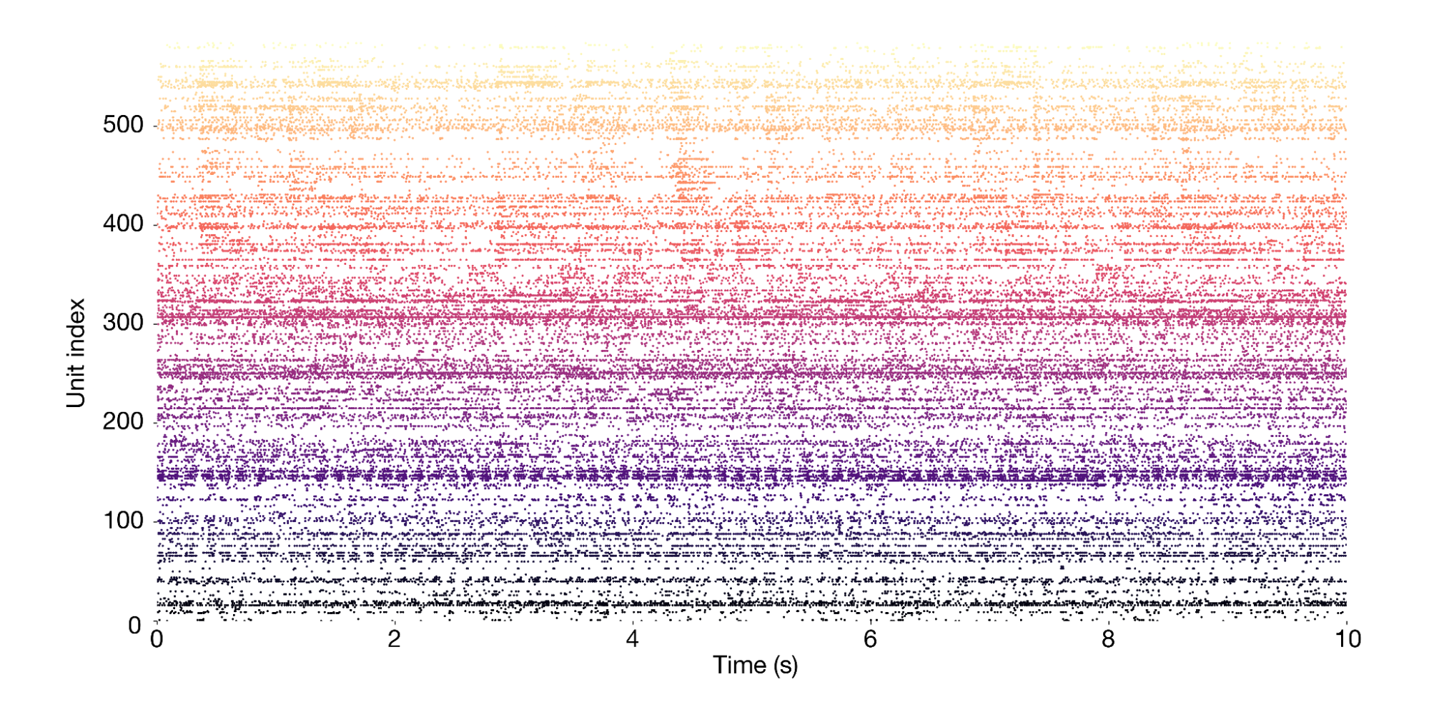
The session object provides access to the primary data, which consists of spike times from 585 neurons (also called "units") simultaneously recorded across more than a dozen brain regions. This is what a 10-second snippet of the recording looks likes, with each dot representing one spike:

Our session object can also be used to access information about the visual stimuli that were shown, the behavior of the mouse, and the electrodes that were used. For example, session.stimulus_presentations returns a DataFrame of all the visual stimuli, with each stimulus indexed by a unique ID. More information about this class can be found in the AllenSDK documentation.

To begin to search for patterns in this data, it's helpful to align spikes to salient events that occur during the session. Since most of these neurons were recorded from visual areas of the mouse brain, they display robust increases in spike rate in response to images and movies. To make it easy to align spikes to a block of stimulus presentations, the EcephysSession class includes a helpful method called presentationwise_spike_counts that takes a time interval, a list of presentation IDs, and a list of unit IDs, and returns an xarray.DataArray containing the binned spiking responses:

1stimulus_presentations = session.stimulus_presentations
2flash_presentations = stimulus_presentations[
3    stimulus_presentations.stimulus_name == "flashes"
4]
5
6responses = session.presentationwise_spike_counts(
7    np.arange(0, 0.5, 0.001),
8    flash_presentations.index.values,
9    session.units.index.values,
10)
11responses.coords
12
Copy

Out:
Coordinates:
  * stimulus_presentation_id         (stimulus_presentation_id) int64 3647 .....
  * time_relative_to_stimulus_onset  (time_relative_to_stimulus_onset) float64 ...
  * unit_id                          (unit_id) int64 951134160 ... 951148915
Copy

This creates a 3-dimensional DataArray with dimensions of stimulus presentation ID, time relative to stimulus onset, and unit ID. We can take the mean along the stimulus presentation axis to generate a plot of the average response for all neurons, with lighter colors indicating a larger response. The plot makes it clear that different neurons respond at different times, and many neurons display an equally large response to both the onset and offset of the stimulus:

1da = responses.mean(dim='stimulus_presentation_id').sortby("unit_id").transpose()
2da.plot(cmap='magma', vmin=0, vmax=0.1)
3
Copy

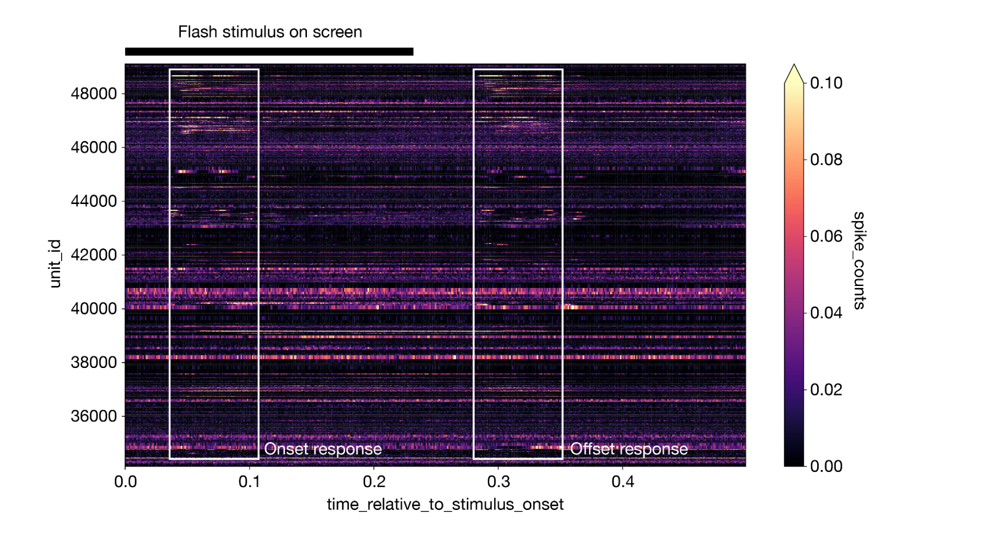
(Note that this figure includes some annotations that were not produced by da.plot().)

Using a DataArray instead of a NumPy ndarray makes it easy to sort, average, and plot large matrices without having to manually keep track of what each axis represents.

In the AllenSDK, we also use Xarray to represent continuous signals from individual electrodes, known as "local field potentials" or “LFP.” We can use the EcephysSession object to load the LFP data for one probe as a DataArray, which makes it straightforward to select time slices of interest:

1lfp = session.get_lfp(session.probes.index.values[0])
2lfp.coords
3
Copy

Out:
Coordinates:
  * time     (time) float64 3.677 3.678 3.679 ... 9.844e+03 9.844e+03 9.844e+03
  * channel  (channel) int64 850297212 850297220 ... 850297964 850297972
Copy

Let's look at the LFP data for a similar segment of data we plotted earlier:

1lfp.sel(time=slice(100,101)).transpose().plot(cmap='magma')
2
Copy

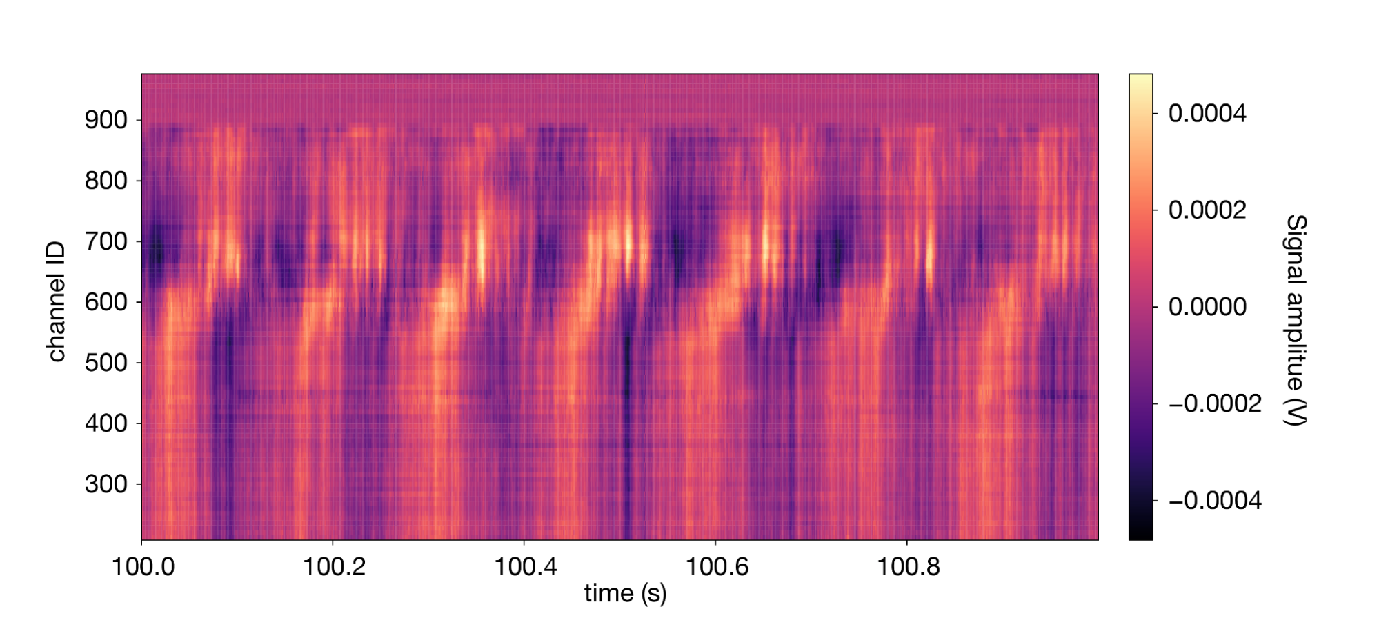
The signal is dominated by a high-amplitude 7 Hz oscillation known as the “theta rhythm.”

The AllenSDK doesn't include a built-in function for aligning LFP to visual stimuli, but this only takes a few lines of code using Pandas and Xarray together:

1presentation_times = flash_presentations.start_time.values
2presentation_ids = flash_presentations.index.values
3
4trial_window = np.arange(0, 0.5, 1 / 500)
5time_selection = np.concatenate([trial_window + t for t in presentation_times])
6
7inds = pd.MultiIndex.from_product(
8    (presentation_ids, trial_window),
9    names=("presentation_id", "time_relative_to_stimulus_onset"),
10)
11
12ds = lfp.sel(time=time_selection, method="nearest").to_dataset(name="aligned_lfp")
13ds = ds.assign(time=inds).unstack("time")
14
15aligned_lfp = ds["aligned_lfp"]
16aligned_lfp.coords
17
Copy

Out:
Coordinates:
  * presentation_id                  (presentation_id) int64 3647 3648 ... 3796
  * time_relative_to_stimulus_onset  (time_relative_to_stimulus_onset) float64 ...
  * channel                          (channel) int64 850297212 ... 850297972
Copy

Now, it only takes one line of code to plot the average response across the whole probe:

1aligned_lfp.mean(dim='presentation_id').plot(cmap='magma')
2
Copy

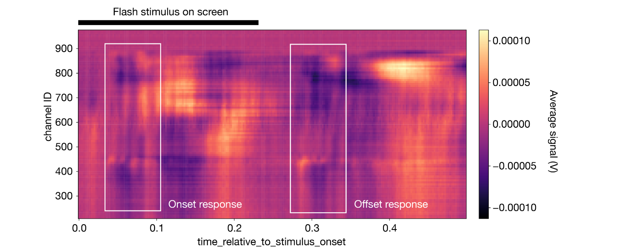
(Note that this figure includes some annotations that were not produced by da.plot().)

The impact of the stimulus is perhaps less obvious here, but the trained eye can see a clear onset and offset response, similar to what was observed in the spiking data.

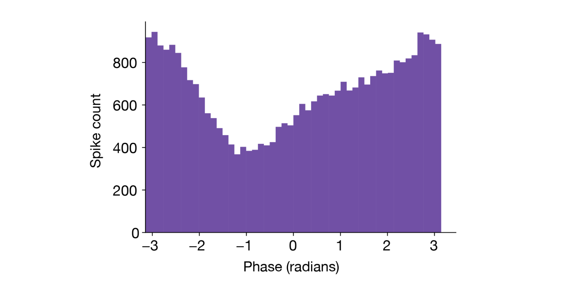
Finally, it's worth mentioning that Xarray also simplifies analyses that relate spikes to LFP. For example, finding the preferred phase of the theta oscillation at which a neuron fires spikes can be done easily using a Hilbert transform and Xarray's sel method:

1from scipy.signal import butter, filtfilt, hilbert
2
3unit_id = units[
4    (units.probe_description == "probeA") & (units.ecephys_structure_acronym == "CA1")
5].index.values[26]
6nearby_lfp = lfp.sel(channel=units.loc[unit_id].peak_channel_id, method="nearest")
7
8b, a = butter(3, np.array([5, 9]) / (1250 / 2), btype="bandpass")
9lfp_filt = filtfilt(b, a, hippocampal_lfp)
10lfp_phase = xr.DataArray(np.angle(hilbert(lfp_filt)), coords={"time": nearby_lfp.time})
11
12spike_phase = lfp_phase.sel(time=session.spike_times[unit_id], method="nearest")
13
Copy

A histogram of the spike phase shows this neuron has a clear preference for the “trough” of theta (±π radians):

Summary#

The Allen Brain Observatory ecephys datasets have been quite popular across the community, with over 50 publications or preprints based on this resource appearing in the last 4 years⁵. We expect that most people are accessing the data via the AllenSDK, which may provide their first exposure to the Xarray library. We hope they appreciate Xarray’s ability to facilitate complex data manipulations without the need to write custom methods.

We are now working on incorporating some of the most useful functions from the AllenSDK into a separate lightweight analysis package. We plan to make all of the return types DataFrames or DataArrays, so they can be easily manipulated using these classes’ powerful built-in methods. While it’s still very early stages, we are excited to continue to build analysis tools on top of the powerful Xarray library.

Acknowledgments#

Special thanks to Nile Graddis for introducing me to Xarray and writing the AllenSDK methods described here. Thanks to Joe Hamman for providing feedback on this post.

References#

1. Stevenson & Körding (2011) Nat Neurosci 14: 139-142.
2. Jun et al. (2017) Nature 551: 232-236.
3. Demas et al. (2021) Nat Methods 18: 1103-1111.
4. Rübel et al. (2022) eLife 11: e78362.
5. De Vries et al. (2023) arXiv 2212.08638.